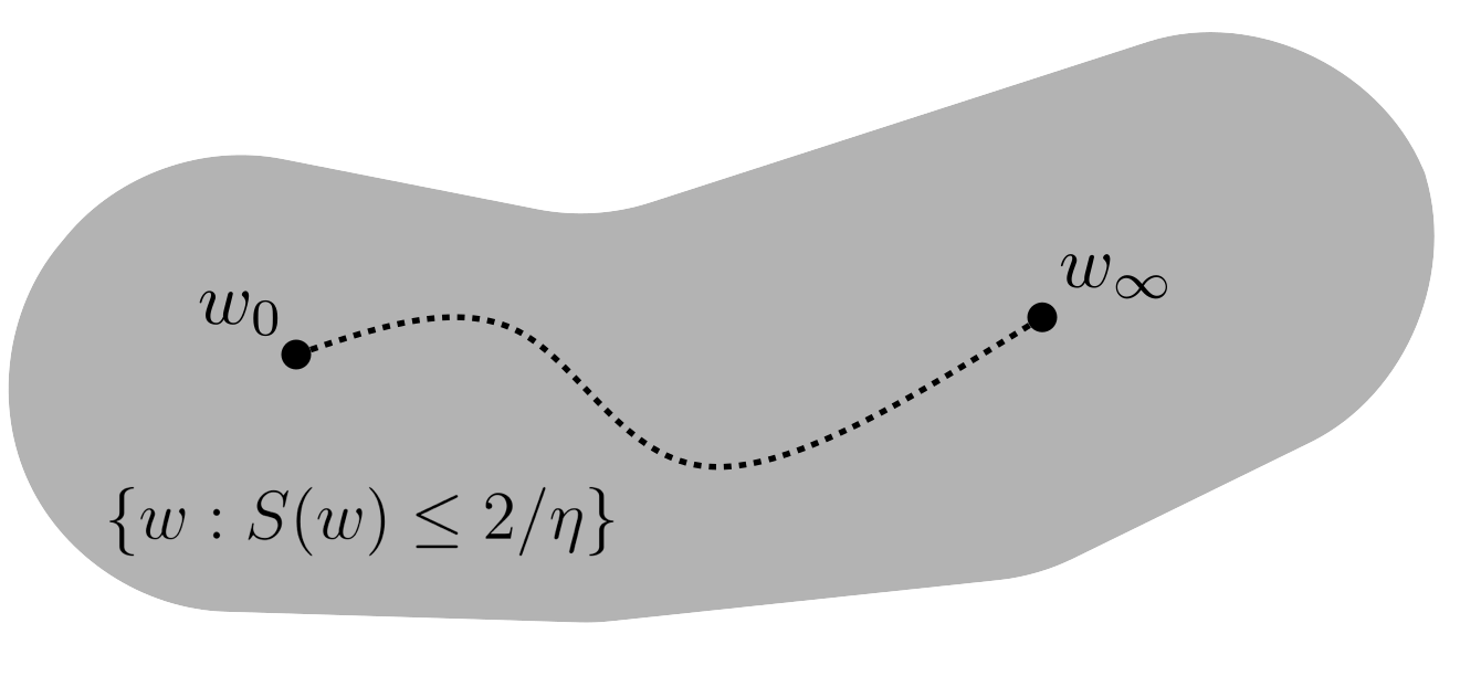
The traditional perspective is that gradient descent remains throughout training inside the "stable region", i.e. the subset of weight space where \(S(w) \le 2/\eta\), visualized here as a gray blob.
This is the companion website for the paper Understanding Optimization in Deep Learning with Central Flows, published at ICLR 2025.
The simplest optimization algorithm is deterministic gradient descent:
Perhaps surprisingly, traditional analyses of gradient descent cannot capture the typical dynamics of gradient descent in deep learning. We'll first explain why, and then we'll present a new analysis of gradient descent that does apply in deep learning.
Let's start with the picture that everyone has likely seen before. Suppose that we run gradient descent on a quadratic function \( \frac{1}{2} S x^2\), i.e. a smiley-face parabola. The parameter \(S\) controls the second derivative ("curvature") of the parabola: when \(S\) is larger, the parabola is steeper.
If we run gradient descent on this function with learning rate \(\eta\), there are two possible outcomes. On the one hand, if \(S < 2/\eta\), then the parabola is "flat enough" for the learning rate \(\eta\), and gradient descent will converge. On the other hand, if \(S > 2/\eta\), then the parabola is "too sharp" for the learning rate \(\eta\), and gradient descent will oscillate back and forth with increasing magnitude.
The same is true for a quadratic function in multiple dimensions. On a multi-dimensional quadratic, the eigenvalues of the Hessian matrix quantify the curvature along the corresponding eigenvectors. If any Hessian eigenvalue exceeds the threshold \(2/\eta\), then this means that the quadratic is "too sharp" in the corresponding eigenvector direction, and gradient descent will oscillate along that direction with increasing magnitude.
Ok, that's quadratics, but what about deep learning objectives? Well, on an arbitrary deep learning objective \(L(w)\), we can always take a quadratic Taylor approximation around our current location in weight space. It's reasonable to think that the dynamics of gradient descent on this quadratic function might resemble the short-term dynamics of gradient descent on the real neural objective. As we've seen, the dynamics of gradient descent on this quadratic are controlled by the largest eigenvalue of the Hessian matrix \(H(w)\), which we will call the sharpness \(S(w)\): \[S(w) := \lambda_1(H(w)).\] Namely, if \(S(w) > 2/\eta\), we know that gradient descent on the quadratic Taylor approximation would oscillate and blow up along the top Hessian eigenvector(s). This argument suggests that gradient descent cannot function properly in regions of weight space where \(S(w) > 2/\eta\).
In light of this discussion, why does gradient descent work in deep learning? Perhaps the most natural explanation is that gradient descent stays in regions of weight space where the sharpness \(S(w)\) is less than \(2/\eta\). In other words, if we define the "stable region" as the subset of weight space where the sharpness is less than \(2/\eta\), then perhaps gradient descent stays inside the stable region throughout training, as in the following cartoon:
Indeed, this is the picture suggested by traditional optimization theory (this is "local L-smoothness").
Yet, as we will now see, the reality in deep learning is quite different. Let's train a neural network using gradient descent with \(\eta = 0.02\). This network happens to be a Vision Transformer trained on a subset of CIFAR-10, but you'd see a similar picture with basically any neural network on any dataset.
As we train, we'll plot the evolution of the sharpness \(S(w)\). Watch what happens:
You can see that the sharpness \(S(w)\) rises until it reaches the threshold \(2/\eta\). This means that gradient descent has left the stable region. At this point, we know that gradient descent would diverge if it were run on the local quadratic Taylor approximation to the training objective, as there is now a direction that is "too sharp" for the learning rate \(\eta\). But, what will happen on the real objective? Let's see.
For the next few iterations of training, we'll plot the train loss and sharpness (as before), but also the displacement of the iterate along the top Hessian eigenvector, i.e. the quantity that is predicted to oscillate.
As you can see, gradient descent does indeed oscillate with growing magnitude along the top Hessian eigenvector, just as a quadratic Taylor approximation would predict. These oscillations eventually grow large enough that the train loss starts to go up instead of down.
Things seem to be going poorly. Will gradient descent succeed? It's not clear how it can: so long as the sharpness exceeds \(2/\eta\), a quadratic Taylor approximation predicts that gradient descent will continue to oscillate with ever-increasing magnitude along the top eigenvector direction.
Let's see what happens over the next few steps of training:
As if by magic, the sharpness drops. And it drops below \(2/\eta\), which is just what we needed to happen. Once the sharpness falls below \(2/\eta\), the oscillations shrink, as we'd expect from taking a new quadratic Taylor approximation. Similarly, the loss comes back down, which is also to be expected. But a key question remains: why did the sharpness conveniently drop, just when we needed it to?
Before we answer this question, let's take a look at the complete training run:
You can see that after rising to \(2/\eta\), the sharpness ceases to grow further, and instead equilibrates around that value. Meanwhile, the training loss behaves non-monotonically over the short-term, while decreasing consistently over the long term.
If we try another learning rate, say \(\eta = 0.01\), then the same thing happens:
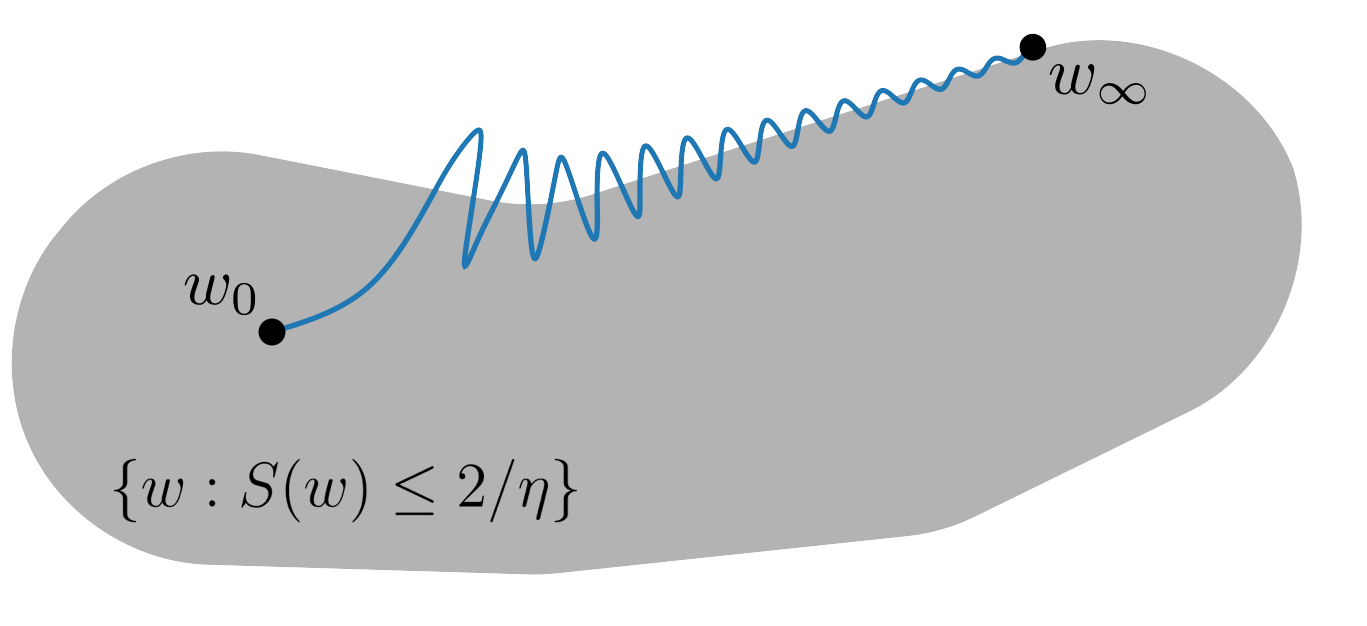
These dynamics are quite surprising. If the traditional picture is that gradient descent remains inside the stable region throughout training, then the reality is that gradient descent is frequently exiting the stable region, but is somehow steering itself back inside each time.
We call these dynamics training at the edge of stability (EOS). This behavior is not specific to this network; rather, as far as anyone can tell, it is a universal phenomenon in deep learning. For example, here are several vision architectures trained using gradient descent on a subset of CIFAR-10:
And here are several sequence architectures trained using gradient descent on a sequence prediction task:
Now, practical loss curves don't look quite like this — for example, they don't usually have such exaggerated loss spikes. That's because practical training usually uses stochastic optimization, whereas this is deterministic gradient descent. We study gradient descent because, as the simplest optimizer, understanding gradient descent would seem to be a necessary stepping stone to understanding SGD. Similar phenomena do occur during SGD and in fact, the study of related phenomena was first pioneered by Stanisław Jastrzębski in the context of SGD.
Several years ago, one of us (Jeremy) wrote a paper which showed that gradient descent exhibits these EOS dynamics, and posed the question:
In response, the other of us (Alex) co-wrote a paper that gave an explanation. It turns out that the key to understanding these gradient descent dynamics is to consider a third-order Taylor expansion of the objective, which is one order higher than is normally used when analyzing gradient descent. A third-order Taylor expansion reveals the key ingredient missing from traditional optimization theory:

Let's sketch this argument informally. Suppose that gradient descent is oscillating along the top Hessian eigenvector, \(u\). Let \(\overline{w}\) denote the point where we'd be if we were not oscillating. But because we are oscillating, the current iterate \(w\) is displaced from \(\overline{w}\) along the direction \(u\) by some magnitude, call it \(x\). Thus the iterate is at: \[ w = \overline{w} + x u\]
How does the gradient at \(w\), where we are, compare to the gradient at \(\overline{w}\), where we'd be if we weren't oscillating? Let's do a Taylor expansion of \(\nabla L\) around \(\overline{w}\). The first two terms of this Taylor expansion are: \[ \nabla L(\overline{w} + xu) = \overset{\textcolor{red}{\text{first term}\strut\strut\strut}}{\nabla L(\overline{w})} + \overset{\textcolor{red}{\text{second term}\strut\strut\strut}}{ \underbrace{x H(\overline{w}) u}_{\textcolor{red}{=\, x S(\overline{w}) u}} } + \mathcal{O}(x^2) \]
Since \(u\) is an eigenvector of the Hessian \( H(\overline{w}) \) with eigenvalue equal to the sharpness \(S(\overline{w})\), the second term can be simplified as \(x H(\overline{w}) u = x S(\overline{w}) u\), which is a vector pointing in the \(u\) direction. This term causes a negative gradient step computed at \(\overline{w} + xu\) to move in the \(-u\) direction. That is, this term is causing us to oscillate back and forth along the top Hessian eigenvector, as predicted by the classical theory.
The "magic" comes from the next term in the Taylor expansion: \[ \nabla L(\overline{w} + xu) = \textcolor{gray}{ \overset{\textcolor{gray}{\text{first term}\strut\strut\strut}}{\nabla L(\overline{w})} + \overset{\textcolor{gray}{\text{second term}\strut\strut\strut}}{ x S(\overline{w}) u }} +\overset{\textcolor{red}{\text{third term}\strut\strut\strut}}{ \underbrace{\frac{1}{2} x^2 \nabla_{\overline{w}} \left[ u^T H(\overline{w}) u \right]}_{\textcolor{red}{= \frac{1}{2} x^2 \nabla S(\overline{w})}} } + \mathcal{O}(x^3) \]
This term looks a little intimidating at first, but let's unpack it. The quantity \( u^T H(\overline{w}) u \) is the curvature in the \(u\) direction. The gradient of this quantity, \(\nabla_{\overline{w}} [u^T H(\overline{w}) u ]\), is the gradient of the curvature in the \(u\) direction. Since \(u\) is the top Hessian eigenvector, the curvature in the \(u\) direction is the top Hessian eigenvalue, i.e. the sharpness. Similarly, it can be shown that the gradient of this curvature is the gradient of the sharpness.
Thus, when gradient descent is oscillating along the top Hessian eigenvector with magnitude \(x\), the gradient automatically picks up a term \( \frac{1}{2} x^2 \nabla S(\overline{w}) \) which points in the direction of gradient of the sharpness, \(\nabla S(\overline{w})\). As a result, each negative gradient step on the loss implicitly takes a negative gradient step on the sharpness of the loss, with the "step size" \(\frac{1}{2} \eta x^2 \). Thus, oscillations automatically reduce sharpness, and the strength of this effect is proportional to the squared magnitude of the oscillation \( x^2 \).
Equipped with this new insight, we can finally understand the behavior of gradient descent that we previously observed:
When gradient descent leaves the stable region, it starts to oscillate with growing magnitude along the top Hessian eigenvector. At first, these oscillations are small, so their effect on the sharpness is negligible. But the oscillations soon grow large enough to exert a non-negligible sharpness-reduction effect. This acts to decrease the sharpness, pushing gradient descent back into the stable region, after which point the oscillations shrink.
In effect, a third-order Taylor approximation reveals that gradient descent has in-built negative feedback mechanism for regulating sharpness: when the sharpness \(S(w)\) exceeds \(2/\eta\), gradient descent oscillates, but the precise effect of such oscillations is to reduce ... the sharpness \(S(w)\)!
In the special case where there is exactly one eigenvalue at the edge of stability, the EOS dynamics consist of consecutive cycles of the kind we just saw, where the sharpness first rises above, and then is pushed below, the value \(2/\eta\):
However, it is common for more than one eigenvalue to eventually reach the edge of stability. The dynamics with multiple eigenvalues at EOS are more complex, and may be chaotic in the technical sense. When there are \(k\) eigenvalues at the edge of stability, gradient descent oscillates within the span of the corresponding \(k\) eigenvectors, and these oscilations cause all \(k\) eigenvalues to stay dynamically regulated around the value \(2/\eta\):
While these dynamics are challenging to analyze, the key insight of our new paper is that understanding the EOS dynamics in fine-grained detail may not be necessary. Rather, we argue that the more important question is: what macroscopic path does gradient descent take through weight space? The goal of our analysis will be to derive a differential equation called a central flow that characterizes this path.
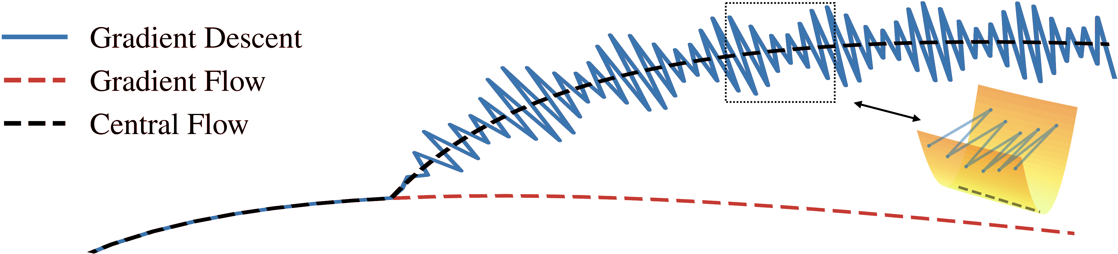
The usual continuous-time approximation to gradient descent is the gradient flow: \[ \begin{align} \frac{dw}{dt} = - \eta \, \nabla L(w), \label{eq:gradient-flow} \end{align} \] Gradient descent roughly follows the gradient flow before reaching the edge of stability. But after reaching EOS, gradient descent splits off from gradient flow, and takes a different path through weight space, as shown in the following animation:
The reason is that gradient flow never oscillates, and hence allows the sharpness to keep rising beyond \(2/\eta\), whereas gradient descent undergoes oscillations which keep the sharpness regulated around \(2/\eta\).
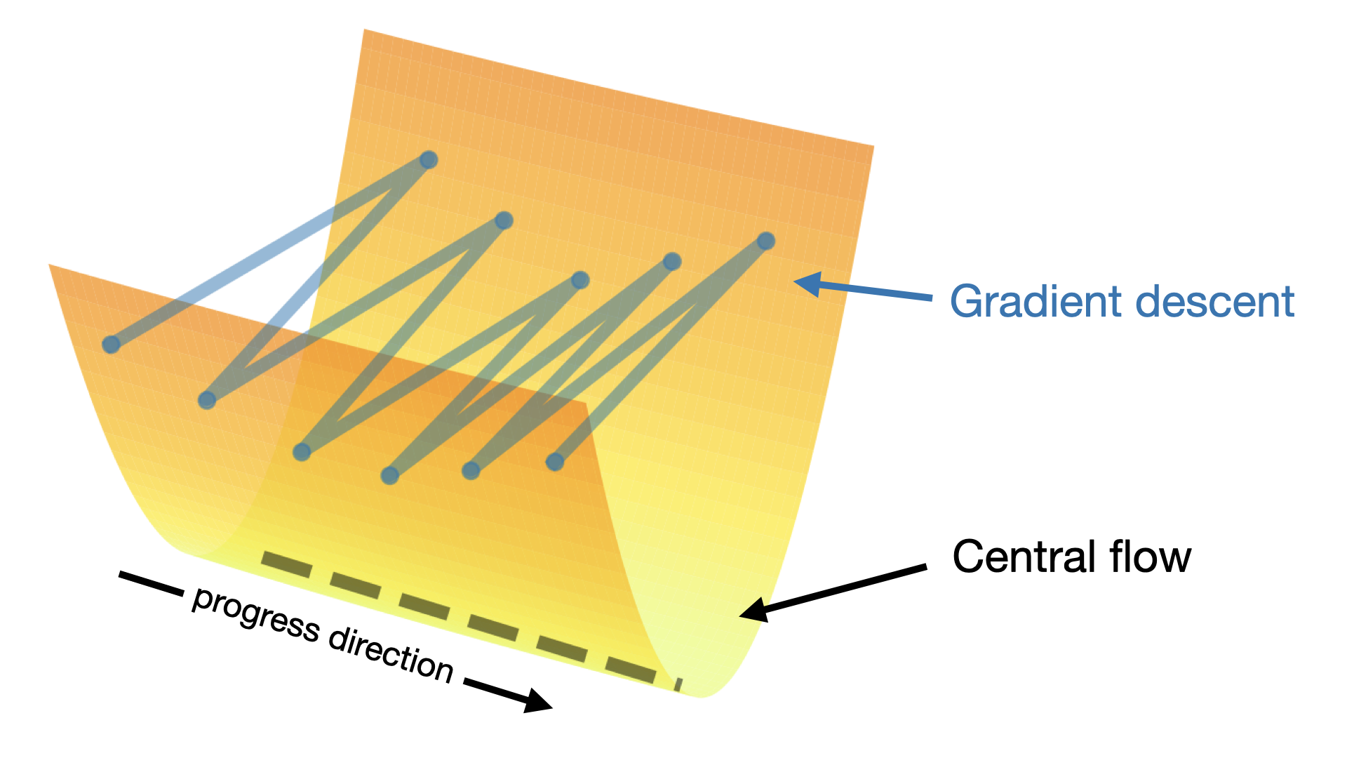
Our central flow is a differential equation that characterizes the trajectory of gradient descent even at the edge of stability. The central flow is depicted by a black dashed line in the following animation:
The central flow models the time-averaged (i.e. locally smoothed) trajectory of gradient descent, as illustrated in the following cartoon of the weight-space dynamics:
We'll derive the central flow using informal mathematical reasoning, and we will then validate its accuracy experimentally. Essentially, our logic proceeds as follows: (1) We will assume that the time-averaged trajectory of gradient descent can be captured by a differential equation. (2) We will argue that only one differential equation makes sense (the central flow). (3) Finally, we will show empirically that this central flow does indeed match the long-term trajectory of gradient descent in a variety of deep learning settings.
Rigorously establishing that gradient descent follows the central flow is an important open problem that is beyond the scope of our paper. Such an analysis would require making assumptions about the objective that we would not know how to justify, and would demand analytical tools that go beyond the usual toolkit of optimization theory. We hope that our compelling experimental results will inspire future efforts aimed at establishing a rigorous basis for similar analyses.
Let's start our derivation by considering the special case where only one eigenvalue is at the edge of stability. The central flow \(w(t)\) will model the time-averaged iterates of gradient descent. Since gradient descent oscillates along the top Hessian eigenvector \(u(t)\), we model each iterate as: \[ \underset{\color{red} \text{iterate}}{w_t} = \underset{\color{red} \begin{array}{c} \text{time-averaged} \\[-4pt] \text{iterate} \end{array} }{w(t)} + \underset{\color{red} \begin{array}{c} \text{perturbation along} \\[-4pt] \text{top eigenvector} \end{array} }{x_t \, u(t)}. \]
Therefore, by Taylor expansion, the gradient at the iterate is: \[ \underset{\color{red} \begin{array}{c} \text{gradient at} \\[-4pt] \text{iterate} \end{array}}{\nabla L(w_t)} \approx \underset{ \color{red} \begin{array}{c} \text{gradient at time-} \\[-4pt] \text{averaged iterate} \end{array}}{\nabla L(w(t))} + \underset{\color{red} \text{oscillation}}{x_t S(w(t)) u(t)} + \underset{\color{red} \text{sharpness reduction}}{\tfrac{1}{2} x_t^2 \nabla S(w(t))}. \]
Therefore, if we abuse notation and use \(\mathbb{E}\) to denote "averages over time", then the "time-averaged" gradient is: \[ \underset{\color{red} \begin{array}{c} \text{time-averaged} \\[-4pt] \text{gradient} \end{array}}{\mathbb{E}[\nabla L(w_t)]} \approx \underset{ \color{red} \begin{array}{c} \text{gradient at time-} \\[-4pt] \text{averaged iterate} \end{array} }{\nabla L(w(t))} + \underset{\color{red} \text{0 because } \mathbb{E}[x_t] = 0 \text{ }}{\color{red}{\cancel{\color{black} \mathbb{E}[x_t] \, S(w(t)) u(t)}}} + \underset{\color{red} \text{implicit sharpness penalty}}{\frac{1}{2} \mathbb{E} [x_t^2] \, \nabla S(w(t))}. \]
That is, the time-averaged gradient equals the gradient at the time-averaged iterate, plus a term proportional to the gradient of the sharpness. The latter scales with \(\mathbb{E} [x_t^2]\), the time-average of the squared magnitude of the oscillations, i.e. the variance of the oscillations. The larger the oscillations, the stronger the induced sharpness penalty.
Based on this calculation, we make the ansatz that the time-averaged dynamics of gradient descent can be captured by a sharpness-penalized gradient flow that follows this time-averaged gradient: \[\begin{align} \frac{dw}{dt} = - \eta \, \left[ \nabla L(w) + \underbrace{\frac{1}{2} \sigma^2(t) \nabla S(w)}_{\color{red} \text{sharpness penalty}} \right], \label{eq:central-flow-ansatz-one-unstable} \end{align}\]
where \(\sigma^2(t)\) is a still-unknown quantity that models the "instantaneous variance" of the oscillations at step \(t\). Intuitively, this flow averages out the oscillations themselves, while retaining their lasting effect on the trajectory, which takes the form of the sharpness penalty.
To set \(\sigma^2(t)\), we will argue that there is only one possible value that it can take. At EOS, the sharpness \(S(w)\) is equilibrating at \(2/\eta\), and is consequently invariant over time. Therefore, we will require that the time derivative of the sharpness along the central flow is zero. It turns out that there is a unique value of \(\sigma^2(t)\) that is compatible with this equilibrium condition.
To see why, note that the time derivative of the sharpness under a flow of the form \eqref{eq:central-flow-ansatz-one-unstable} is given by: \[ \begin{align} \frac{dS}{dt} &= \left \langle \nabla S(w), \frac{dw}{dt} \right \rangle \tag{chain rule} \\[0.4em] &= \left \langle \nabla S(w), - \eta \, \left[ \nabla L(w) + \frac{1}{2} \sigma^2(t) \nabla S(w) \right] \right \rangle \tag{ansatz for $\tfrac{dw}{dt}$} \\[0.4em] &= \underset{\color{red} \begin{array}{c} \text{time derivative of sharpness} \\[-4pt] \text{under gradient flow} \end{array}}{\left \langle \nabla S(w), - \eta \nabla L(w) \right \rangle} - \underset{\color{red} \begin{array}{c} \text{sharpness reduction} \\[-4pt] \text{from oscillations} \end{array} }{\tfrac{1}{2} \eta \, \sigma^2(t) \| \nabla S(w) \|^2}. \tag{simplify} \end{align} \]
The first term is the time derivative of the sharpness under gradient flow, which will be positive (as otherwise we would have left the edge of stability). The second term is the sharpness reduction that is induced by the oscillations. Basic algebra shows that there is a unique value of \(\sigma^2(t)\) for which the second term cancels the first term to yield \(\frac{dS}{dt} = 0\), and this is given by:
\[ \begin{align} \sigma^2(t) = \frac{2 \langle -\nabla L(w), \nabla S(w) \rangle }{\| \nabla S(w)\|^2}. \label{eq:sigma-squared-one-unstable} \end{align} \]
The central flow is defined as equation \eqref{eq:central-flow-ansatz-one-unstable}, with this particular value of \(\sigma^2(t)\) plugged in: \[ \begin{align} \frac{dw}{dt} = - \eta \, \left[ \nabla L(w) + \frac{1}{2} \sigma^2(t) \nabla S(w) \right] \quad \text{where}\quad \sigma^2(t) = \frac{2 \langle -\nabla L(w), \nabla S(w) \rangle }{\| \nabla S(w)\|^2}. \label{eq:central-flow-one-unstable} \end{align} \]
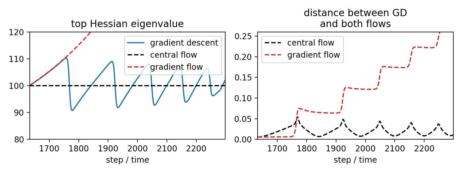
Let's check out this central flow in action. Starting at the point in training where the sharpness first reaches \(2/\eta\), we'll run both gradient descent and the central flow \eqref{eq:central-flow-one-unstable} side by side:
The left pane shows that the sharpness cycles around \(2/\eta\) under gradient descent, and stays fixed at exactly \(2/\eta\) under the central flow. This is not particularly interesting, since we constructed the central flow specifically to have this property. What is more interesting are the other two panes.
The middle pane shows that our formula \eqref{eq:sigma-squared-one-unstable} for \(\sigma^2(t)\) can accurately predict the instantaneous variance of the oscillations. In light blue, we show the squared magnitude of the displacement between gradient descent and the central flow along the top Hessian eigenvector, and in thick blue we compute the empirical time-average of this quantity, i.e. the empirical variance of the oscillations (we use Gaussian smoothing). Observe that the central flow's \(\sigma^2(t)\), in black, accurately predicts this quantity.
The right pane shows that the gradient descent stays close to the central flow over time. In particular, it shows that the Euclidean distance between these two processes remains small. In contrast, the figure below shows that the distance between gradient descent and the gradient flow starts to grow large once training enters EOS:
Thus, although our analysis utilizes informal mathematical reasoning, we can see that this analysis yields precise, nontrivial numerical predictions about the optimization dynamics.
So far, we have focused on the special case where only one eigenvalue is at the edge of stability. But the central flow formalism extends more generally to the setting where an arbitrary number of eigenvalues can be at the edge of stability (including zero). In general, we model gradient descent as displaced from its time-averaged trajectory \(w(t)\) by some perturbation \(\delta_t\) that lies within the span of the unstable eigenvectors: \[ \underset{\color{red} \text{iterate}}{w_t} = \underset{\color{red} \begin{array}{c} \text{time-averaged} \\[-4pt] \text{iterate} \end{array} }{w(t)} + \underset{\color{red} \begin{array}{c} \text{perturbation} \end{array} }{\delta_t}. \]
Going through a similar argument as before, we arrive at the ansatz that the time-averaged iterates of gradient descent follow a flow of the form: \[ \begin{align} \frac{dw}{dt} = - \eta \left[ \nabla L(w) \, + \,\underbrace{\tfrac{1}{2} \nabla_w \langle H(w), \Sigma(t) \rangle}_{\color{red} \text{penalize \(\Sigma\)-weighted Hessian}} \right], \label{eq:central-flow-ansatz-multi-unstable} \end{align} \] where \(\Sigma(t)\ := \mathbb{E}[\delta_t \delta_t^T]\) models the instantaneous covariance matrix of the oscillations. Here, \(\langle \cdot, \cdot \rangle \) denotes the trace inner product between two matrices, so the quantity \(\langle H(w), \Sigma(t) \rangle\) is a linear combination of the entries of the Hessian, where each entry is weighted by the corresponding entry of \(\Sigma(t)\). The flow implicitly penalizes this quantity, to capture the effect on the time-averaged trajectory of oscillations with covariance \(\Sigma(t)\).
As before, to determine \(\Sigma(t)\), we argue that only one value "makes sense." Namely, we impose three conditions on the flow:
It turns out that there is a unique value of \(\Sigma(t)\) satisfying all three conditions, and it can be found by solving a convex program called a semidefinite complementarity problem (SDCP). The central flow is defined as equation \eqref{eq:central-flow-ansatz-multi-unstable} with this particular value of \(\Sigma(t)\) plugged in. Note that when the sharpness is below \(2/\eta\), the SDCP will always return \(\Sigma(t) = 0\), and so the central flow will reduce to the gradient flow.
Let's now watch the central flow in action:
Initially, all Hessian eigenvalues are below \(2/\eta\), so \(\Sigma(t) = 0\), and the central flow reduces to the gradient flow. After the top Hessian eigenvalue reaches \(2/\eta\), \(\Sigma(t)\) becomes rank-one, and the central flow keeps the top eigenvalue locked at \(2/\eta\), as it mimics the effects of oscillating along the the top eigenvector direction. After the second Hessian eigenvalue also reaches \(2/\eta\), \(\Sigma(t)\) becomes rank-two, and the central flow keeps the top two eigenvalues both locked at \(2/\eta\), as it mimics the effects of oscillating simultaneously along the top two eigenvector directions.
On the right, observe that the distance between the gradient descent and the central flow stays small over time, whereas the distance between gradient descent and gradient flow starts to grow large once the dynamics enter EOS. (The red line ends early because we stop discretizing gradient flow once the sharpness gets high enough that discretization becomes too challenging.)
Now for the coolest part, in our subjective opinion. As before, we can verify that our prediction \(\Sigma(t)\) does indeed accurately model the instantaneous covariance matrix of the oscillations. In particular, we can see that each eigenvalue of \(\Sigma(t)\) accurately predicts the instantaneous variance of oscillations along the corresponding eigenvector of \(\Sigma(t)\):
We think this is really cool. While the oscillations appear to be chaotic, they obey a hidden underlying order — namely, their covariance is predictable. Moreover, the long-term trajectory of gradient descent only depends on the oscillations via this covariance. Thus, we don't need to understand the exact oscillations to understand the long-term path taken by gradient descent — we just need to understand their covariance, which is much easier.
OK, so we've shown that the central flow takes the same long-term path as gradient descent. But, one might ask, if they're the same, then why is one better? Well, as a smooth curve, the central flow is a fundamentally simpler object than the oscillatory gradient descent trajectory. For example, under the gradient descent trajectory, the network's predictions evolve erratically, due to the oscillations:
By contrast, since the central flow is a smooth curve, everything (including the network's predictions) evolves smoothly under the central flow:
Philosophically, we think of the central flow as the "true" training process, and we regard the actual gradient descent trajectory as merely a "noisy" approximation to this true underlying process.
In particular, let's use the central flow perspective to understand something that every deep learning practitioner is familiar with: the train loss curve. Here's what a typical gradient descent loss curve looks like:
As you can see, the loss behaves non-monotonically over short-timescales, while only decreasing over long-timescales. This makes it challenging to reason about the progress of optimization.
In contrast, the central flow's loss curve \(L(w(t))\) is much nicer:
In fact, it is possible to prove that the central flow decreases the loss monotonically: \( \frac{d}{dt} L(w(t)) \leq 0 \). Thus, the loss along the central flow \(L(w(t))\) is a hidden progress metric, or potential function, for the optimization process.
As you can see above, the loss along the central flow is consistently lower than the loss along the gradient descent trajectory. The intuitive explanation is that at EOS, gradient descent can be viewed as "bouncing between valley walls", whereas the central flow moves nearly along the "valley floor." The loss is higher on the valley walls, when gradient descent is located, than on the valley floor, where the central flow is located.
Fortunately, because the central flow models the covariance \(\Sigma(t)\) with which gradient descent oscillates around the central flow, it can render predictions for the time-averaged train loss along the gradient descent trajectory: \[ \underset{\color{red} \begin{array}{c} \text{time-averaged} \\[-4pt] \text{train loss} \end{array}}{\mathbb{E}[L(w_t)]} = \underset{\color{red} \begin{array}{c} \text{loss at} \\[-4pt] \text{central flow} \end{array}}{L(w(t))} + \underset{\color{red} \begin{array}{c} \text{contribution from} \\[-4pt] \text{oscillations} \end{array}}{\frac{1}{\eta} \text{tr}(\Sigma(t))} \]
The following animation shows that this prediction is quite accurate:
The loss along the central flow \(L(w(t))\) is roughly analogous to the loss evaluated at an exponential moving average of the recent weights, whereas the prediction for the time-averaged train loss \(L(w(t)) + \tfrac{1}{\eta} \text{tr}(\Sigma(t))\) is roughly analogous to the smoothed training loss curve.
The same principle applies to the gradient norm. The gradient norm along the central flow is much smaller than the gradient norm along the gradient descent trajectory, since most of the latter is dominated by the back-and-forth oscillations "across the valley" that cancel out over the long run. Nevertheless, by leveraging \(\Sigma(t)\), the central flow can predict the time-averaged gradient norm of gradient descent:
Although this post has focused on a particular ViT as a running example, we stress that our analysis is fully generic, and applies across a variety of architectures and tasks. For example, here we show real vs. predicted loss curves for a variety of deep learning settings:
Please see the paper for a discussion of the circumstances under which the central flow is a good approximation to gradient descent.
Interested in this line of work? Consider pursuing a PhD with Alex Damian, who will join the MIT Math and EECS departments in Fall 2026.