When \(S_{\text{eff}} > 2\), Scalar RMSProp "bounces up the walls" of the valley.
This is the companion website for the paper Understanding Optimization in Deep Learning with Central Flows, published at ICLR 2025.
Adaptive optimizers such as Adam are a widely used class of optimization algorithms in deep learning. These optimizers dynamically adjust their step sizes in response to recent gradients. Yet, despite the ubiquity of these algorithms, many questions remain unanswered, including perhaps the most basic: what, precisely, does the optimizer adapt to?
In this section, we will study a simple adaptive optimizer, termed Scalar RMSProp:
\[ \underset{\color{red}{\text{maintain EMA of squared gradient norm}\rule[20pt]{0pt}{0pt}}}{\nu_{t} = \beta_2 \, \nu_{t-1} + (1-\beta_2) \|\nabla L(w_t)\|^2}, \quad \quad \underset{\color{red}{\text{take gradient step of size } \eta / \sqrt{\nu}}}{ w_{t+1} = w_t - \frac{\eta}{\sqrt{\nu_{t}}} \nabla L(w_t)}. \]
As its name suggests, this is a scalar-valued version of RMSProp. Whereas RMSProp adapts one step size for each parameter, Scalar RMSProp adapts a single global step size. In particular, the algorithm maintains an exponential moving average, \(\nu_t\), of the squared gradient norm, and then takes gradient steps using the effective step size \(\eta / \sqrt{\nu_{t}}\).
Our analysis will clarify the precise sense in which Scalar RMSProp "adapts" its effective step size \(\eta / \sqrt{\nu_t} \) to the local loss landscape. We will see that although the optimizer explicitly uses the gradient, it really adapts to the curvature. But that's not all: as we'll see, Scalar RMSProp also has a hidden mechanism for shaping the curvature along its trajectory, and this mechanism is crucial for the optimizer's ability to optimize quickly.
These points will extend to RMSProp in Part III, but are simpler to understand for Scalar RMSProp.
Let's start by watching Scalar RMSProp in action. Here's the first part of the trajectory:
Starting around step 90, the gradient norm starts to spike regularly, and the network's predictions start to oscillate. What happened? Scalar RMSProp has entered an oscillatory edge of stability regime:
To understand why Scalar RMSProp oscillates, recall from Part I that gradient descent with step size \(\eta\) oscillates along the top Hessian eigenvector(s) if the sharpness \(S(w)\) exceeds the threshold \(2/\eta\). One can view Scalar RMSProp as gradient descent with the dynamic step size \(\eta / \sqrt{\nu_t}\). Accordingly, we expect Scalar RMSProp to oscillate whenever the sharpness \(S(w)\) exceeds \(\sqrt{\nu_t} \, (2 / \eta)\). Equivalently, if we define the effective sharpness as \[S_{\text{eff}} := \eta \, S(w) / \sqrt{\nu_t},\] then we expect Scalar RMSProp to oscillate whenever \(S_{\text{eff}}\) exceeds the critical threshold \(2\).
The key to understanding the dynamics we just saw is to examine the evolution of the effective sharpness \(S_{\text{eff}}\):
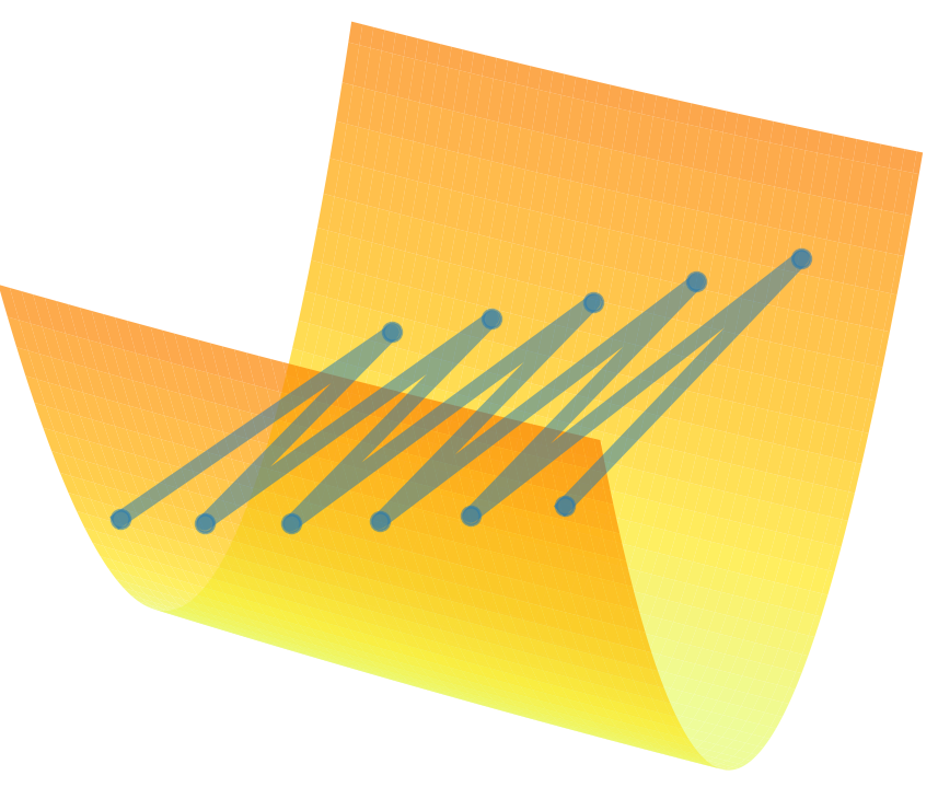
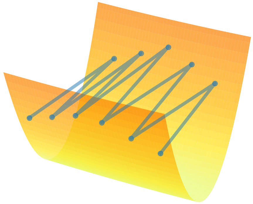
So long as the effective sharpness \(S_{\text{eff}}\) is less than 2, the optimizer is stable. But soon enough, \(S_{\text{eff}}\) rises above 2, due to growth in both the sharpness \(S(w_t)\) and the effective step size \(\eta / \sqrt{\nu_t}\). Once \(S_{\text{eff}} > 2\) the optimizer starts to oscillate in weight space along the top Hessian eigenvector. Visually, such oscillations can be visualized as "bouncing up the walls" of a valley:
These oscillations cause the network's predictions to oscillate, and the gradient norm to rise. Yet, the oscillations do not trigger divergence, because they induce reduction in the effective sharpness, as we will discuss momentarily. This negative feedback re-stabilizes the system, causing the oscillations to shrink.
The net result is that the effective sharpness equilibrates around the value 2, as the optimizer oscillates without diverging along the top Hessian eigenvector(s). We refer to this regime as training at the edge of stability.
For Scalar RMSProp, there are two separate mechanisms by which oscillations induce reduction of the effective sharpness \(S_{\text{eff}}\). First, as with gradient descent, oscillations automatically trigger reduction of sharpness \(S(w_t)\), decreasing \(S_{\text{eff}}\) via its numerator. But Scalar RMSProp also possesses an additional mechanism for stabilizing itself: oscillations increase the gradient norm, causing \(\nu_t\) to grow, which reduces the effective sharpness \(S_{\text{eff}}\) via its denominator. Both of these mechanisms play a role in stabilizing Scalar RMSProp, as can be seen in the following animation:
The hyperparameter \(\beta_2\) has a subtle effect on these dynamics, because it controls the speed at which the EMA \(\nu\) can react to the growth in the gradient norm. Watch what happens if we try a larger value of \(\beta_2 = 0.999\), which makes \(\nu\) slower to adapt:
You can see that for the larger value of \(\beta_2\), at the end of the spike, \(\nu \) has grown less, and the sharpness \(S(w)\) has dropped more. Intuitively, Scalar RMSProp is leaning more on sharpness reduction, and less on \(\nu\) adaptation, to stabilize itself. Indeed, over the long run, different values of \( \beta_2 \) can result in very different trajectories:
The cycles you see above — where the effective sharpness first rises above, then falls below, the value 2 — typify the dynamics in the special case where there is just one eigenvalue at the edge of stability. Even in this relatively simple setting, the dynamics are challenging to analyze, as one must account for the mutual interactions between the sharpness, the oscillations, and the EMA \(\nu\).
Things get even more complex in the more common setting when multiple eigenvalues have reached the edge of stability. With multiple eigenvalues at EOS, Scalar RMSProp oscillates simultaneously along all the corresponding eigenvectors, and all such eigenvalues stay regulated around 2:
Fortunately, as with gradient descent, we will see that while it may be hard to analyze the exact trajectory, it is surprisingly easy to characterize the time-averaged (i.e. locally smoothed) trajectory of Scalar RMSProp. We will now derive a central flow that captures this time-averaged trajectory.
When Scalar RMSProp is stable, it approximately tracks the following differential equation, which we call the stable flow (see the paper for the explanation for this expression): \[ \begin{align} \frac{dw}{dt} = -\frac{\eta}{\sqrt{\nu}} \nabla L(w), \quad \quad \frac{d \nu}{dt} = \frac{1-\beta_2}{\beta_2} \left( \|\nabla L(w)\|^2 - \nu \right). \label{eq:stable-flow} \end{align} \]
However, once Scalar RMSProp enters the edge of stability, it deviates from the stable flow \eqref{eq:stable-flow} and takes a different path through weight space:
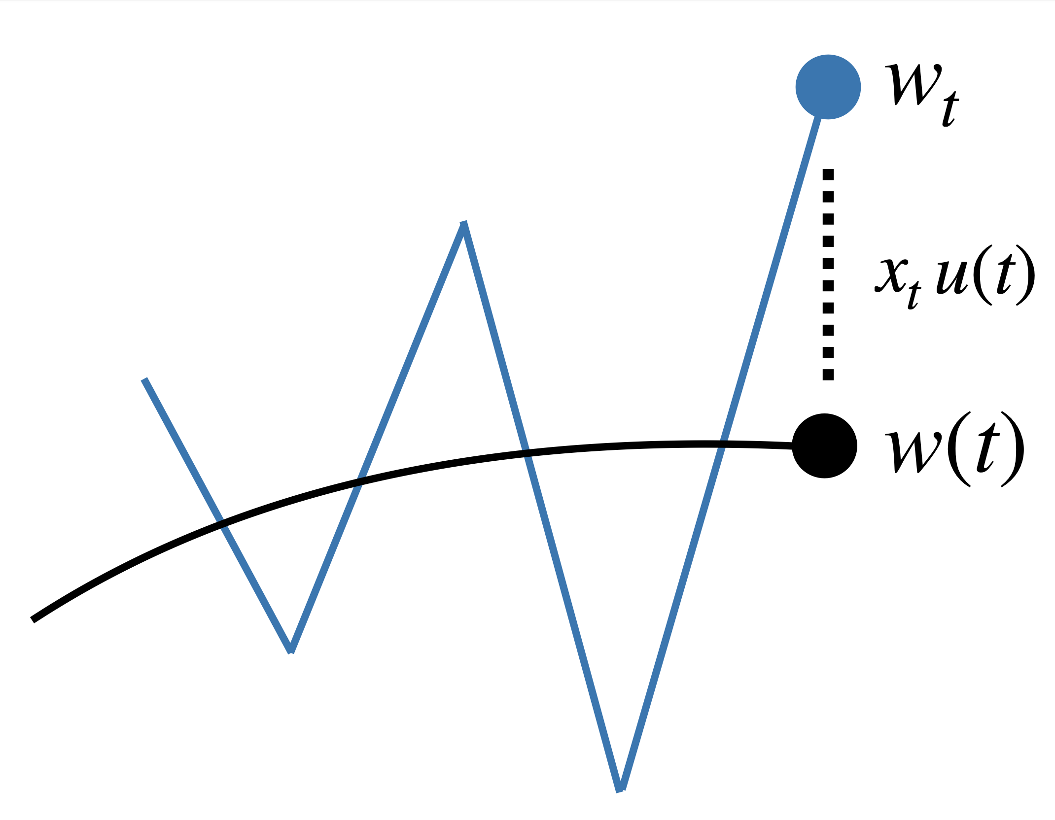
Our central flow \(w(t)\) will characterize this path. For now, let us consider the case where just one eigenvalue is at the edge of stability. As before, we model the iterate \(w_t\) as being displaced from the time-averaged iterate \(w(t)\) by some perturbation along the top Hessian eigenvector \(u(t)\) with magnitude \(x_t\):
\[ w_t = w(t) + x_t \, u(t). \]
In Part I, we computed that the time-averaged gradient is then given by: \[ \underset{\color{red} \begin{array}{c} \text{time-averaged} \\ \text{gradient} \end{array}}{\mathbb{E}[\nabla L(w_t)]} \approx \underset{\color{red} \begin{array}{c} \text{gradient at time-} \\ \text{averaged iterate} \end{array}}{\nabla L(w(t))} + \underset{\color{red} \begin{array}{c} \text{implicit sharpness} \\ \text{reduction} \end{array}}{\tfrac{1}{2} \mathbb{E}[x_t^2] \nabla S(w(t))}. \]
Similarly, by using the first two terms in the Taylor expansion of \(\nabla L\), we can approximate the time-average of the squared gradient norm as: \[ \underset{\color{red} \begin{array}{c} \text{time-averaged} \\[-0.2em] \text{gradient norm}^2 \end{array}}{\mathbb{E}[\|\nabla L(w_t)\|^2]} \approx \underset{\color{red} \begin{array}{c} \text{gradient norm}^2 \text{ at time-} \\ \text{averaged iterate} \end{array}}{\|\nabla L(w(t))\|^2} + \underset{\color{red} \begin{array}{c} \text{contribution from} \\ \text{oscillations} \end{array}}{\mathbb{E}[x_t^2] \, S(w(t))^2}. \]
Based on these time-averages, we make the ansatz that the time-averaged dynamics of \(w, \nu \) can be captured by a central flow \(w(t), \nu(t) \) of the following functional form: \[ \begin{align} \frac{dw}{dt} = -\frac{\eta}{\sqrt{\nu}} \underbrace{\left[ \nabla L(w) + \frac{1}{2} \sigma^2(t) \nabla S(w) \right]}_{\color{red}{\text{time-averaged gradient}}}, \quad \quad \frac{d \nu}{dt} = \frac{1-\beta_2}{\beta_2} \left[ \underbrace{ \| \nabla L(w) \|^2 + \sigma^2 (t) S(w)^2}_{\color{red}{\text{time-averaged gradient norm}^2}} - \nu \right], \label{eq:ansatz} \end{align} \]
where \(\sigma^2(t)\) is a still-unknown quantity that models the instantaneous variance of the oscillations at time \(t\).
As with gradient descent, to determine \(\sigma^2(t)\), we observe that the effective sharpness \(S_{\text{eff}}\) equilibrates at the value 2, and is consequently invariant over time. Based on this, we will require that the time derivative of \(S_{\text{eff}}\) along the central flow should be equal to zero. It turns out that there is a unique value of \(\sigma^2(t)\) that is compatible with this equilibrium condition (the formula is in the paper). The central flow is given by eq. \eqref{eq:ansatz} with this \(\sigma^2(t)\).
The resulting flow accurately captures the complex dynamics of Scalar RMSProp that we saw earlier:
Thus, a remarkably simple time-averaging argument has allowed us to characterize the long-term trajectory of a complex dynamical system.
As described in the paper, this derivation can also be extended to the more general setting where an arbitrary number of eigenvalues are at EOS, including zero. When there are no eigenvalues at EOS, the central flow reduces to the stable flow eq. \eqref{eq:stable-flow}.
We empirically show in the paper that this central flow can accurately capture the dynamics of Scalar RMSProp across a variety of deep learning settings. For example, the following figure illustrates how we can accurately predict the time-averaged loss curves:
Let us now use the central flow formalism to understand precisely how Scalar RMSProp "adapts" its effective step size to the local loss landscape.
For Scalar RMSProp, the effective step size \(\eta / \sqrt{\nu_t}\) fluctuates rapidly, due to the oscillations. By contrast, along the central flow, the effective step size \(\eta / \sqrt{\nu(t)}\) evolves smoothly:
In fact, at the edge of stability, we can say more about the central flow's effective step size. At EOS, the effective sharpness \(S_{\text{eff}} := \eta \, S(w) / \sqrt{\nu}\) stays fixed at 2. Since \(S_{\text{eff}}\) is the product of the effective step size \( \eta / \sqrt{\nu} \) and the sharpness \( S(w) \), this implies that the effective step size \( \eta / \sqrt{\nu} \) must always be equal to \(2 / S(w)\). In other words, although the sharpness \(S(w(t))\) is gradually changing, \(\nu(t)\) must be changing commensurately so that the effective step size \( \eta / \sqrt{\nu(t)} \) always stays fixed at \(2 / S(w(t))\):
Notably, the value \(2 / S(w)\) is the largest stable step size for gradient descent at the location \(w\). Thus, we see that Scalar RMSProp automatically keeps the effective step size tuned to the largest stable step size, even as this value evolves through training. This is the precise sense in which the algorithm is "adaptive."
Of course, you could invent an optimizer that manually computes the sharpness \(S(w)\) at each step, and manually sets the step size to \(2 / S(w)\). But this would involve some extra computation. What is interesting is that Scalar RMSProp does the same thing efficiently, requiring only one gradient query per iteration — the same cost as a step of gradient descent. This rich behavior is implicit in the optimizer's oscillatory dynamics. Thanks to these oscillatory dynamics, an optimizer that accesses the loss only via gradients is able to adapt to the local Hessian.
Further, note that even comprehending this step size strategy requires an appeal to some notion of time averaging. The effective step size of Scalar RMSProp is not exactly fixed at \(2/S(w(t))\), but rather fluctuates around this value. The important thing is that it is \(2/S(w(t))\) on average over time. The central flow perspective allows us to reason about this behavior.
So, is that all there is to it? Should we think of Scalar RMSProp as just an efficient method for online estimation of the maximum stable step size? No, there is something missing from this picture: to fully understand Scalar RMSProp's behavior, we must account for the sharpness reduction effect that is induced by the oscillations. To quantify this effect, we can return to the central flow. In general, the central flow is a joint flow over \((w(t), \nu(t))\). But at EOS, because \( \eta / \sqrt{\nu(t)} = 2 / S(w(t)) \), we can eliminate \(\nu\) from the picture, and write the central flow as a flow over \(w\) alone:
\[ \frac{dw}{dt} = -\underset{\color{red} \text{adapt step size}}{\frac{2}{S(w)}} {\left[ \nabla L(w) + \underset{\color{red} \text{implicitly reduce sharpness}}{\frac{1}{2} \sigma^2(w; \eta, \beta_2) \nabla S(w)} \right]} \]
This is saying that at EOS, Scalar RMSProp is effectively equivalent to the following simpler-to-understand algorithm:
It can be analytically shown that the sharpness regularizer \(\sigma^2(w; \eta, \beta_2)\) is monotonically increasing in \(\eta\). That is, larger learning rates lead to larger oscillations, and thus induce stronger sharpness regularization. Indeed, this figure illustrates how larger learning rates take a trajectory with lower sharpness:
In the study of optimization for machine learning, it is common to view questions of sharpness as a generalization concern, separate from the core optimization concern of making the loss go down fast. But it turns out that for Scalar RMSProp, implicitly regularizing sharpness makes training go faster. Why would that be? In the animation below, we compare Scalar RMSProp and its central flow to an ablated flow, \[ \frac{dw}{dt} = -\underset{\color{red} \text{adapt step size}}{\frac{2}{S(w)}} {\left[ \nabla L(w) \right]}, \] which adapts the step size to \(2/S(w)\), but does not also regularize sharpness.
Over time, the ablated flow navigates into regions with higher sharpness \(S(w)\) (center), because it lacks the implicit sharpness regularization that Scalar RMSProp has. In these sharper regions, the effective step size of \(2/S(w)\) is smaller (right), and optimization accordingly proceeds slower (left). In contrast, by regularizing sharpness, Scalar RMSProp is able to steer itself into lower-sharpness regions, where it can and does take larger steps.
Implicit sharpness regularization is also crucial for understanding the function of the learning rate hyperparameter \(\eta\). Recall that at the edge of stability, the effective step size is fixed at \(2/S(w)\). Notably, this value is independent of the learning rate hyperparameter \(\eta\). Thus, the only direct effect of \(\eta\) on the central flow is to modulate the strength of the sharpness regularizer, with higher \(\eta\) inducing stronger sharpness regularization.
But crucially, because stronger sharpness regularization guides the optimizer into lower-sharpness regions where \(2/S(w)\) is larger, a higher \(\eta\) can indirectly enable larger effective step sizes later in training. Thus, even at EOS, larger \(\eta\) can result in larger effective step sizes; but they do so via this subtle, indirect mechanism.
Interested in this line of work? Consider pursuing a PhD with Alex Damian, who will join the MIT Math and EECS departments in Fall 2026.