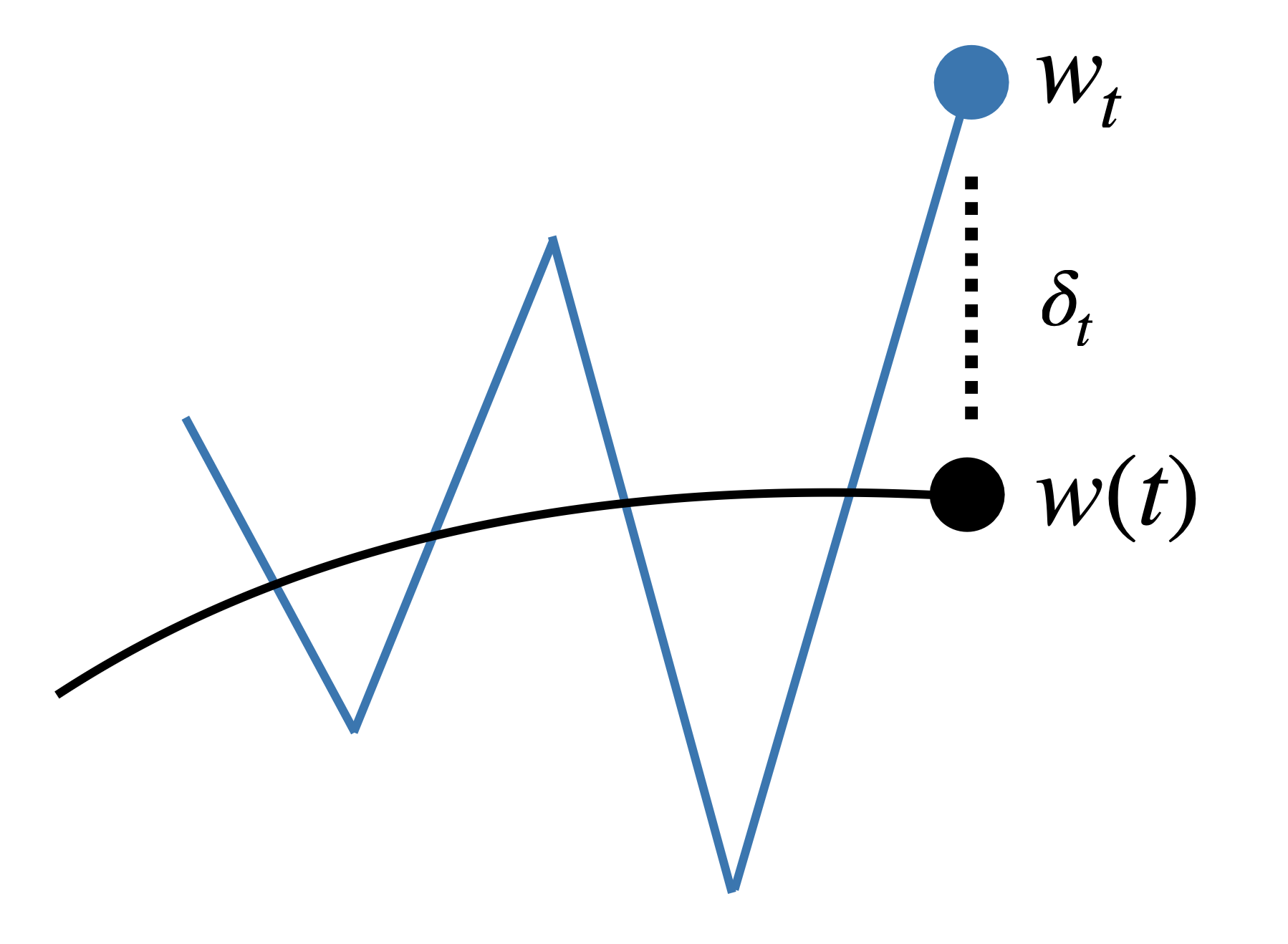
We model the iterate \(w_t\) as displaced from the central flow \(w(t)\) by some oscillation \(\delta_t\)
This is the companion website for the paper Understanding Optimization in Deep Learning with Central Flows, published at ICLR 2025.
We now study RMSProp, which is equivalent to Adam without momentum: \[ \underset{\color{red}{\text{update EMA of squared gradient}\,\rule[18pt]{0pt}{0pt}}} {\nu_{t} = \beta_{2} \, \nu_{t-1} + (1-\beta_{2}) \nabla L(w_t)^{\odot 2}}, \quad \quad \underset{\color{red}{\text{take preconditioned gradient step}}}{w_{t+1} = w_t - \frac{\eta}{\sqrt{\nu_{t}} }\odot \nabla L(w_t)}. \]
RMSProp maintains an exponential moving average (EMA) \(\nu\) of the element-wise squared gradient \(\nabla L(w)^{\odot 2}\), and then takes a step using per-coordinate step sizes of \(\eta / \sqrt{\nu}\). There is an equivalent viewpoint that is sometimes more convenient to work with: if we define preconditioned gradient descent as: \( w_{t+1} = w_t - P^{-1} \nabla L(w_t)\), then RMSProp is preconditioned gradient descent with the dynamic preconditioner \(P_t = \text{diag}(\sqrt{\nu_t} / \eta)\).
Adam uses the same preconditioning strategy, and has achieved massive success in deep learning. However, it is a mystery why this particular preconditioner should work so well. Common folklore is that Adam/RMSProp adapts to the "curvature", i.e. Hessian, of the objective function. However, it is unclear why this should be the case, since Adam/RMSProp updates its preconditioner using the gradient \( \nabla L \), not the Hessian \( \nabla^2 L \).
In this section, we will use the central flows framework to understand RMSProp. We will see that RMSProp does adapt to the local Hessian after all — but the reason is inextricably tied to the optimizer's oscillatory dynamics, which have not been previously studied.
Let's start by getting some intuition for RMSProp's behavior. We'll train a ResNet on a subset of CIFAR-10 using deterministic RMSProp. As you can see, the loss curve looks pretty well-behaved:
Yet, even though it looks like smooth sailing, there are interesting things happening beneath the surface. Recall that RMSProp maintains an EMA \( \nu_t\) of the element-wise squared gradient \( \nabla L(w_t)^{\odot2} \). Let's examine the dynamics of these two quantities at several individual coordinates:
You can see that the entries of the squared gradient \( \nabla L(w_t)^{\odot 2} \) are fluctuating rapidly. This causes their EMA \( \nu_t \) to also fluctuate (although less so). Since this EMA is used to determine the algorithm's step sizes \( \eta / \sqrt{\nu_t} \), we need to understand the origin of this behavior if we want to understand how RMSProp sets its step sizes / preconditioner.
These fluctuations in the gradient arise because, like gradient descent, RMSProp is operating in an oscillatory edge of stability regime. To understand why RMSProp would oscillate, consider running preconditioned gradient descent: \[ w_{t+1} = w_t - P^{-1} \nabla L(w_t) \] on a quadratic function with Hessian \( H \). The resulting dynamics are controlled by the effective Hessian \( P^{-1} H \). If this matrix has any eigenvalue greater than 2, then preconditioned gradient descent will oscillate along the corresponding (right) eigenvector, as illustrated in the animation below:
While deep learning objectives are not globally quadratic, a local quadratic Taylor approximation suggests that RMSProp will oscillate if any eigenvalues of the current effective Hessian \( P_t^{-1} H(w_t) = \text{diag}(\eta / \sqrt{\nu_t}) \, H(w_t) \) exceed the critical threshold 2.
Let's examine how the eigenvalues of the effective Hessian evolve, under the dynamics of RMSProp:
Initially, all eigenvalues are below 2, and the optimizer does not oscillate. Once the top eigenvalue rises to the threshold 2, RMSProp enters an edge of stability regime where optimizer oscillates along the unstable eigenvector(s) of the effective Hessian, and such oscillations induce reduction of the corresponding eigenvalue(s). The net effect is that the top eigenvalues equilibrate around the value 2.
For RMSProp, there are two distinct mechanisms by which oscillations along the unstable eigenvectors reduce the unstable eigenvalues of the effective Hessian \( \text{diag}(\eta / \sqrt{\nu}) \, H(w_t)\). First, such oscillations induce implicit regularization of the Hessian \(H(w_t)\), as is revealed by considering a local cubic Taylor expansion of the objective (recall Part I). Second, such oscillations increase the gradient (as will be made clear below) and hence \(\nu_t\). RMSProp stabilizes itself using a combination of both mechanisms.
While analyzing the exact dynamics is challenging, as in Part I and Part II we will see that analyzing the time-averaged dynamics is much easier.
So long as RMSProp is stable (i.e. all eigenvalues of the effective Hessian are less than 2), its trajectory is reasonably well-approximated by the following differential equation, which we call the stable flow: \[ \begin{align} \frac{dw}{dt} = -\frac{\eta}{\sqrt{\nu}} \nabla L(w), \quad \quad \frac{d \nu}{dt} = \left(\frac{1 - \beta_2}{\beta_2} \right) \nabla L(w)^{\odot 2}. \label{eq:stable-flow} \end{align} \]
Upon reaching the edge of stability, RMSProp starts to oscillate, and deviates from this path. We will now derive a central flow that characterizes the time-averaged trajectory of RMSProp even at EOS.
As in Part I, we model RMSProp \(\{w_t\}\) as being displaced from the central flow \(w(t)\) by some oscillation \(\delta_t\) that lies within the span of the eigenvectors that are at the edge of stability: \[ \underset{\color{red} \text{iterate}}{w_t} = \underset{\color{red} \begin{array}{c} \text{time-averaged} \\[-4pt] \text{iterate} \end{array} }{w(t)} + \underset{\color{red} \begin{array}{c} \text{oscillation} \end{array} }{\delta_t} \quad \text{where} \quad \underset{\color{red} \begin{array}{c} \substack{\; \; \, \delta_t \text{ is eigenvector of effective} \\ \text{Hessian with eigenvalue 2} }\end{array} }{\text{diag}(\eta / \sqrt{\nu}) \, H(w(t)) \, \delta_t = 2 \, \delta_t}. \]
Recall from Part I that the time-averaged gradient is then approximately: \[ \underbrace{\mathbb{E}[\nabla L(w_t)]}_{\color{red}{\substack{\text{time-average} \\ \text{of gradient}}}} \approx \underbrace{\nabla L(w(t))}_{\color{red}{\substack{\text{gradient at time-} \\ \text{averaged iterate}}}} + \underbrace{\tfrac{1}{2} \nabla \langle \Sigma(t), H(w(t)) \rangle}_{\color{red}{\substack{\text{implicit curvature} \\ \text{reduction}}}}, \] where \(\Sigma(t) = \mathbb{E}[\delta_t \delta_t^T] \) models the instantaneous covariance matrix of the oscillations at time \(t\).
We can similarly compute the time-average of the squared gradient, by using the first two terms in the Taylor expansion of \(\nabla L\), and by using that the oscillation \(\delta_t\) is an eigenvector of the effective Hessian with eigenvalue 2: \[ \begin{align} \underbrace{\mathbb{E}[\nabla L(w_t)^{\odot 2}]}_{\color{red}{\substack{\text{time-average of} \\ \text{ squared gradient}}}} \approx \underbrace{\nabla L(w(t))^{\odot 2}}_{\color{red}{\substack{\text{squared gradient at} \\ \text{time-averaged iterate}}}} + \underbrace{ \frac{4 \nu}{\eta^2} \odot \text{diag}[\Sigma(t)] }_{\color{red}{\substack{\text{contribution from oscillations}}}}. \label{eq:time-average-sq-gradient} \end{align} \]
This calculation makes clear that larger oscillations (i.e. larger diagonal entries of \(\Sigma(t)\)) increase the time-averaged squared gradient.
Based on these time-averages, we make the ansatz that the time-averaged dynamics of RMSProp can be captured by a central flow \((w(t), \nu(t)) \) of the following functional form: \[ \begin{align} \frac{dw}{dt} = -\frac{\eta}{\sqrt{\nu}} \odot \left[\underbrace{\nabla L(w) + \tfrac{1}{2} \nabla \langle \Sigma(t), H(w) \rangle}_{\color{red} \text{time-average of gradient} }\right], \quad \quad \frac{d\nu}{dt} = \frac{1-\beta_2}{\beta_2} \left[\underbrace{\nabla L(w)^{\odot 2} + \frac{4\nu}{\eta^2} \odot \text{diag}[\Sigma(t)]}_{\color{red} \text{time-average of squared gradient} } - \nu \right ]. \label{eq:ansatz} \end{align} \] As in Part I, to determine \(\Sigma(t)\), we impose three natural conditions, and show that only one value of \(\Sigma(t)\) satisfies all three conditions. This value is the solution to a certain semidefinite complementarity problem (SDCP). The RMSProp central flow is defined as equation \eqref{eq:ansatz} with this value of \(\Sigma(t)\). Note that this central flow automatically reduces to the stable flow \eqref{eq:stable-flow} when all eigenvalues of the effective Hessian are less than 2.
Let's take a look at the central flow in action. You can see that under the central flow, each eigenvalue of the effective Hessian rises to 2 and then stays locked at this value:
We can furthermore assess whether the central flow's \(\Sigma(t)\) does indeed accurately predict the instantaneous covariance matrix of the oscillations. In particular, we can verify that each eigenvalue of \(\Sigma(t)\) accurately predicts the variance of the oscillations along the corresponding eigenvector of \(\Sigma(t)\). (We actually use generalized eigenvectors/eigenvalues under the preconditioner \(P(t)\).)
Thus, while the exact oscillations may be chaotic and hard to analyze, their time-average is predictable and comparably easy to analyze.
We will now use the central flow to understand how RMSProp implicitly sets its preconditioner.
First, let us revisit the fluctuations in the squared gradient \(\nabla L(w_t)^{\odot 2} \) that we saw earlier. These fluctuations arise due to the oscillations in weight space along the top eigenvectors of the effective Hessian. Since the central flow models the covariance \(\Sigma(t)\) of these oscillations, it can render predictions for the time-average of the squared gradient, \( \mathbb{E}[\nabla L(w_t)^{\odot 2}] \), via equation \eqref{eq:time-average-sq-gradient}. As you can see, this prediction is quite accurate:
Thus, while the precise fluctuations in the squared gradient may be chaotic, their time-average is predictable.
Interestingly, we can see that most of the squared gradient \(\nabla L(w_t)^{\odot 2} \) originates from the oscillations, i.e. the second term of \eqref{eq:time-average-sq-gradient}, rather than from the squared gradient at the time-averaged iterate, i.e. the first term of \eqref{eq:time-average-sq-gradient}. Intuitively, if we recall that an oscillating optimization algorithm can be visualized as moving through a "valley" while bouncing between the "valley walls", then this means that most of the squared gradient comes from the valley walls, rather than from the valley floor.
The central flow can also accurately predict the dynamics of \(\nu\), the EMA of the squared gradient:
In keeping with the broader story, we see that although \(\nu_t\) is rapidly fluctuating, its time-averaged trajectory \(\nu(t)\) is smooth and predictable.
Let us now use the central flow to understand how RMSProp sets its preconditioner. Unfortunately, even at the edge of stability, \(\nu(t)\) cannot always be expressed purely as a function of \(w(t)\) (as it was for Scalar RMSProp in Part II), and instead remains an independent variable that must be tracked. This reflects the fact that for any \(w\), there are potentially many values for \(\nu\) that could stabilize optimization, and the actual value used by RMSProp depends on the historical trajectory.
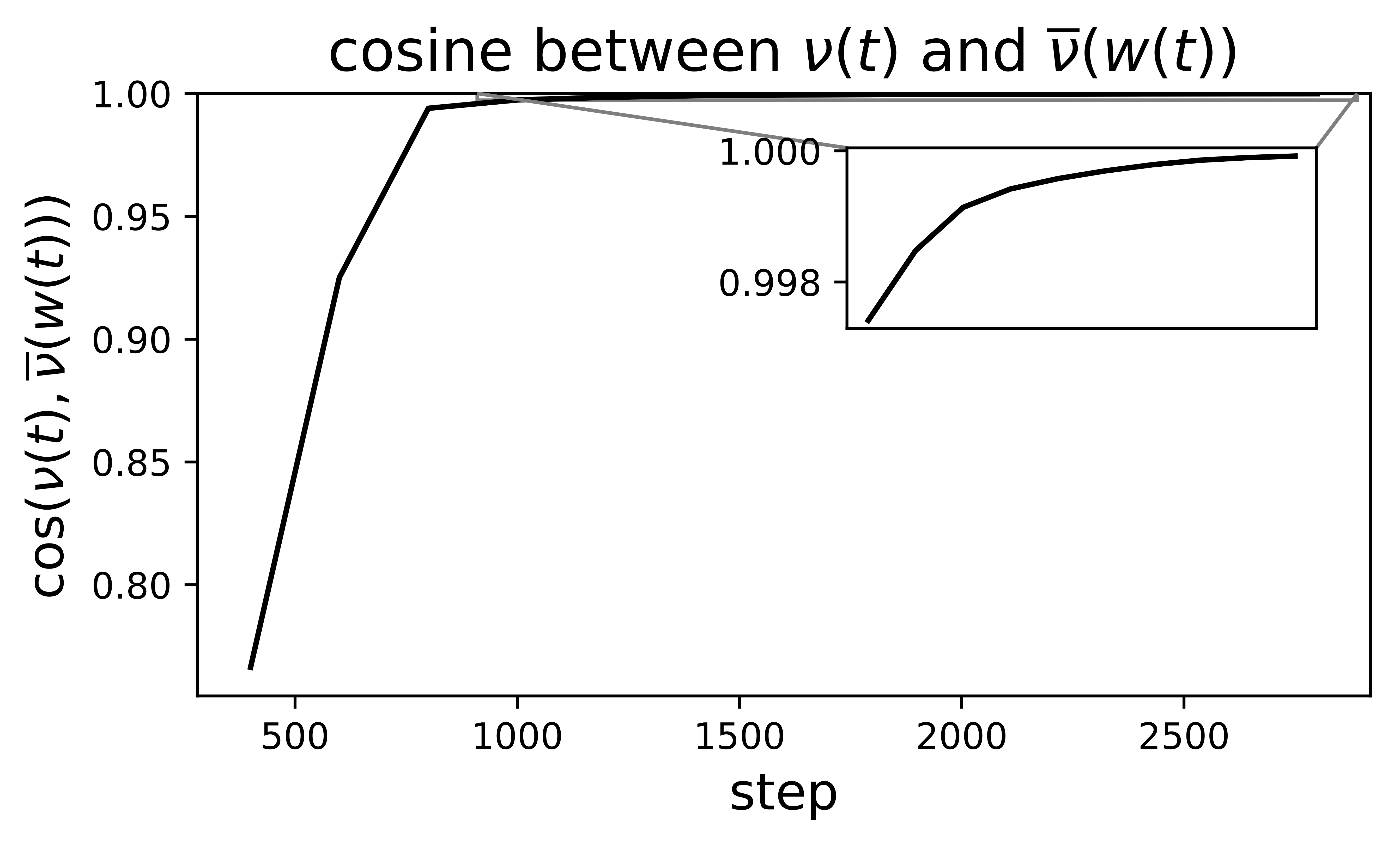
Nevertheless, it turns out that, in some circumstances, \(\nu\) implicitly converges under the dynamics of RMSProp to a value that depends on the current \(w\) alone. For any weights \(w\), imagine freezing \(w\) in place and running the \(\nu\) dynamics until a fixed point is reached. It turns out that for any \(w\), there is always a unique \(\nu\) satisfying the stationarity condition \( \frac{d\nu}{dt} = 0 \). We refer to this unique \(\nu\) as the stationary EMA, denoted \( \overline{\nu}(w) \), for the weights \(w\). We will say more about the stationary EMA momentarily, but first let us verify the relevance of the stationarity argument.
In the figure below, we measure the cosine similarity between the real EMA \(\nu(t)\) and the stationary EMA \(\overline{\nu}(w(t))\) during training by the central flow. You can see that the cosine similarity rises to very high values (near 1), indicating that the real EMA \(\nu(t)\) converges to the stationary EMA \(\overline{\nu}(w(t))\).
We can also see that the real EMA \(\nu(t)\) agrees with the stationary EMA \(\overline{\nu}(w(t))\) on a coordinate-wise level:
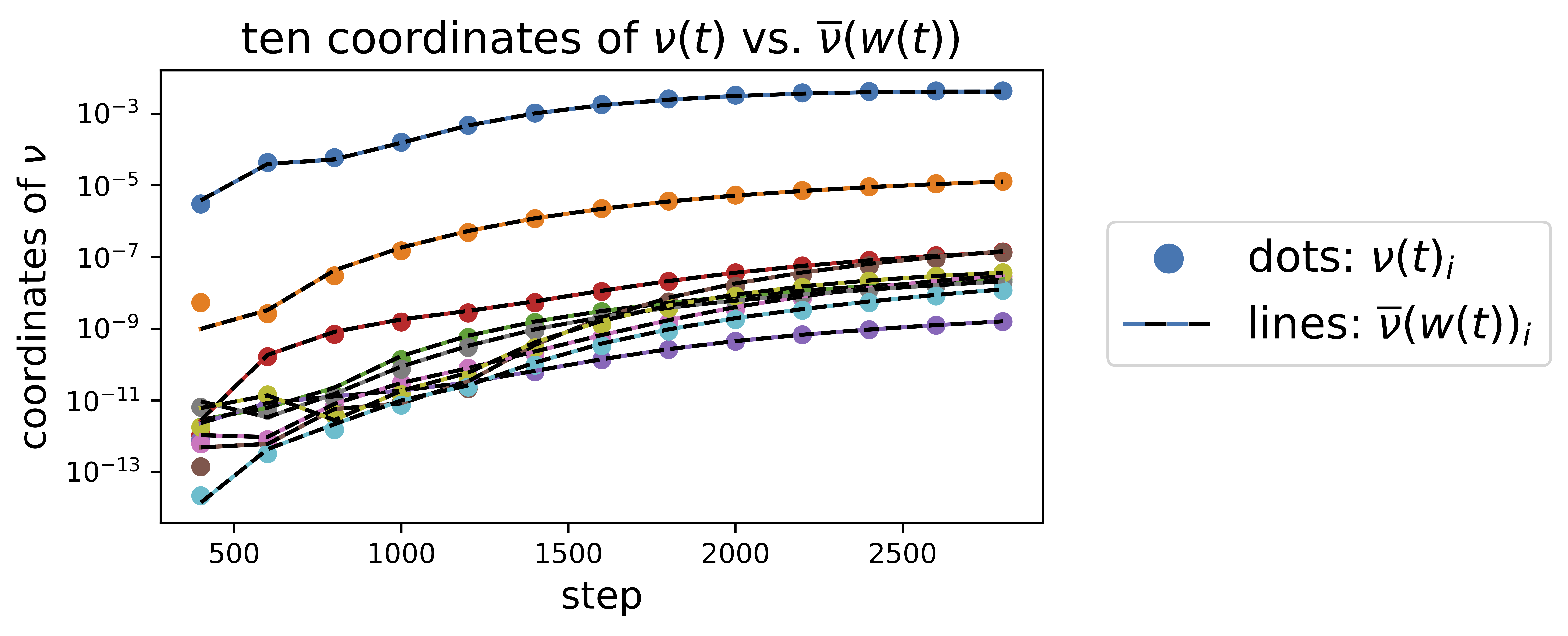
Intuitively, the original central flow describes the simultaneous dynamics of optimization (the \(w\) dynamics), and preconditioner adaptation (the \(\nu\) dynamics). That \(\nu(t)\) is converging to \(\overline{\nu}(w(t))\) implies that the \(\nu\) dynamics of preconditioner adaptation are happening on a faster timescale than the \(w\) dynamics of optimization, so that the adaptive preconditioner is usually "all caught up" with the current weights \(w\).
So, what is the stationary EMA \(\overline{\nu}(w)\)? It is a bit analytically nicer to work in terms of the corresponding stationary preconditioner \( \overline{P}(w) := \frac{\sqrt{\overline{\nu}(w)}}{\eta} \). Remarkably, one can show that this stationary preconditioner is the optimal solution to a convex optimization problem over preconditioners:
\[ \begin{align} \overline{P}(w) = \operatorname*{argmin}_{\substack{P \text{ diagonal}, \; P \succeq 0}} \ \text{trace}(P) + \tfrac{1}{\eta^2} \underbrace{\| \nabla L(w)\|^2_{P^{-1}}}_{\text{optimization speed}} \quad \text{such that} \quad \underbrace{H(w) \preceq 2P}_{\text{local stability}}. \label{eq:convex-program-P} \end{align} \]
That is, RMSProp implicitly solves the convex program \eqref{eq:convex-program-P} to compute its preconditioner. This behavior is implicit in the optimizer's oscillatory dynamics. Our analysis has rendered RMSProp's preconditioning strategy explicit for the first time.
Now that we are able to write down the preconditioner that RMSProp implicitly uses, we can interpret this preconditioner to gain some understanding into RMSProp's preconditioning strategy. The constraint in \eqref{eq:convex-program-P} is equivalent to the stability condition \( P^{-1} H(w) \preceq 2 I \) and hence ensures that the preconditioner keeps RMSProp locally stable. The first term in the objective of \eqref{eq:convex-program-P} is the trace of the preconditioner, or equivalently the sum of the inverse effective learning rates. If this were the only term in the objective, then the optimization problem \eqref{eq:convex-program-P} would reduce to maximizing the sum of the inverse effective learning rates while maintaining local stability:
\[ \begin{align} \hat{P}(w) := \operatorname*{argmin}_{\substack{P \text{ diagonal}, \; P \succeq 0}} \ \text{trace}(P) \quad \text{such that} \quad \underbrace{H(w) \preceq 2P}_{\text{local stability}}. \label{eq:convex-program-P-alternate} \end{align} \]
This is an intuitively sensible preconditioner criterion. What do we want in a preconditioner? Well, we want the effective learning rates to be as large as possible, but we also need local stability, and these two desiderata are in tension. To resolve the tension, if we have some scalar-valued metric for quantifying the "largeness" of the vector of effective learning rates, then we can formulate preconditioner selection as a constrained optimization problem. Minimizing the sum of the inverse effective learning rates (i.e the trace of the preconditioner) is one such metric.
In fact, if the diagonal constraint were not present, and if the Hessian \(H(w)\) were PSD, then we could say more: the optimization problem eq. \eqref{eq:convex-program-P-alternate} would have the closed-form solution \( \hat{P}(w) = \tfrac{1}{2} H(w) \). That is, the preconditioner \(P\) would be a scaling of the Hessian, and preconditioned gradient descent would move in the same direction as Newton's method. Even if the Hessian were not PSD, a similar point would hold — the optimization problem eq. \eqref{eq:convex-program-P-alternate} would have the closed-form solution \( \hat{P}(w) = \tfrac{1}{2} \Pi_{\mathbb{S}_+} H(w) \), where \( \Pi_{\mathbb{S}_+} \) denotes projection onto the cone of positive semidefinite matrices.
With the diagonal constraint present, this argument no longer applies, but we can empirically assess the efficacy of the preconditioner eq. \eqref{eq:convex-program-P-alternate} on deep learning loss functions. To quantify the efficacy of a preconditioner \(P\) at weights \(w\), we can measure the quantity \( \| \nabla L(w) \|^2_{P^{-1}} := \nabla L(w)^T P^{-1} \nabla L(w) \), which is the instantaneous rate of loss decrease under the preconditioned gradient flow. A natural "baseline" preconditioner is the one corresponding to vanilla gradient descent with the maximum locally stable learning rate, i.e. \(P(w) = (2/S(w))^{-1} I\), where \(S(w)\) is the largest Hessian eigenvalue at \(w\).
The figure below shows that, along the RMSProp central flow at various learning rates, the preconditioner eq. \eqref{eq:convex-program-P-alternate} indeed beats this baseline.
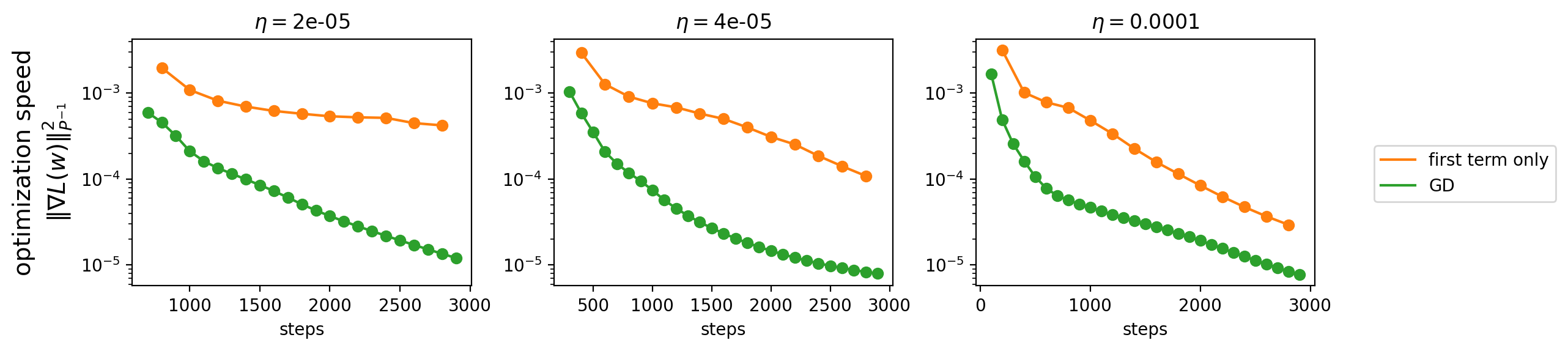
Unfortunately, the second term in the objective of \eqref{eq:convex-program-P} makes matters more complicated. This term is precisely the optimization speed of preconditioned gradient flow with preconditioner \(P\). Minimizing this quantity necessarily acts to slow down optimization, which is bad. Indeed, the figure below shows that RMSProp's stationary preconditioner \eqref{eq:convex-program-P} is always worse than the first-term-only variant \eqref{eq:convex-program-P-alternate}, and is sometimes even worse than our "baseline" of gradient descent:
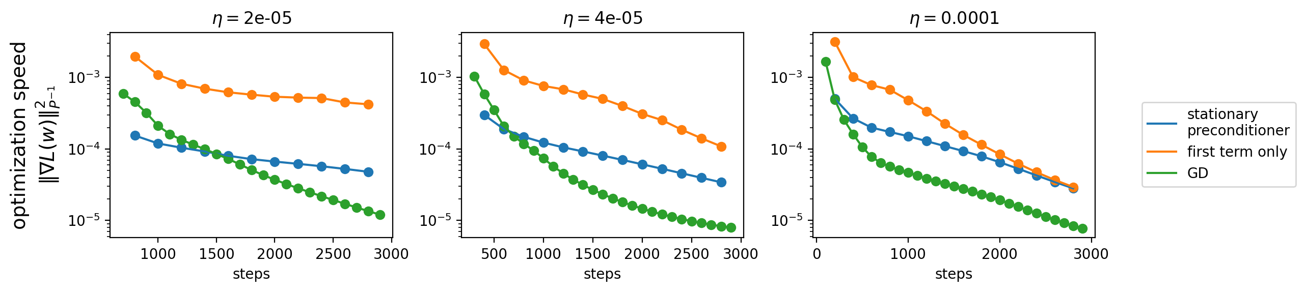
Thus, the second term in eq. \eqref{eq:convex-program-P} is a harmful presence in RMSProp's implicit preconditioning strategy.
In summary, our analysis has rendered explicit the preconditioner eq. \eqref{eq:convex-program-P} that is implicit in RMSProp's oscillatory dynamics. We are not claiming that this preconditioner is optimal in any sense; all we are claiming that this is exactly what RMSProp does, for better or for worse. We believe that understanding this preconditioning strategy is likely a prerequisite for understanding many other aspects of RMSProp's behavior.
So, is that it? Should we think of RMSProp as an algorithm that implicitly performs preconditioned gradient descent using the preconditioner eq. \eqref{eq:convex-program-P}? Not quite — there is one thing missing from this picture. RMSProp is oscillating, and while much of the oscillatory motion cancels out, the oscillations induce a curvature reduction effect which we must account for. To do so, we can return to the central flow.
By substituting the stationary preconditioner \eqref{eq:convex-program-P} into the central flow, we can obtain a stationary flow over \(w\) alone: \[ \begin{align} \frac{dw}{dt} = - \underset{\color{red} \substack{\text{stationary} \\ \text{preconditioner}}}{\overline{P}(w)^{-1}} \odot \left[\nabla L(w) + \underset{ \color{red} \text{implicit curvature penalty} }{\tfrac{1}{2} \nabla \langle \Sigma(t), H(w) \rangle} \right], \label{eq:stationary-flow} \end{align} \]
where \(\Sigma(t)\) is defined as the solution to an SDCP. This flow models the preconditioner as adapting "infinitely fast" to the current weights \(w\), so that we can treat it as always being fixed at its current stationary value. It suggests that we should view RMSProp as performing preconditioned gradient descent, using the preconditioner eq. \eqref{eq:convex-program-P}, not on the original objective but on a certain curvature-penalized objective.
Empirically, we find that the stationary flow \eqref{eq:stationary-flow} is less accurate than the original central flow, but is nevertheless often a decent approximation to the RMSProp trajectory, provided that RMSProp has reached the edge of stability and that the preconditioner has converged to its stationary value.
As with Scalar RMSProp (Part II), we find that the implicit curvature penalty is beneficial for RMSProp's efficacy as an optimizer (i.e. even if we don't care about generalization, and care only about making the loss go down fast). In particular, if we disable the central flow's implicit curvature penalty, then we find that the flow proceeds into higher-curvature regions in which it takes smaller steps, and optimizes slower:
Indeed, in the limit of large \(\eta\), the stationary preconditioner eq. \eqref{eq:convex-program-P} converges to eq. \eqref{eq:convex-program-P-alternate}, which is independent of \(\eta\). Thus, in this limit, the learning rate hyperparameter \(\eta\) has no direct effect on the stationary preconditioner, and only affects the stationary flow via the curvature regularization term. But, as with Scalar RMSProp (Part II), this can give \(\eta\) an indirect effect on the preconditioner later in training.
Interested in this line of work? Consider pursuing a PhD with Alex Damian, who will join the MIT Math and EECS departments in Fall 2026.